Mechanics of Learning
How do neural networks learn? In this post, I consolidate all of the snippets and useful tips that helped me understand neural networks, backpropagation, and other techniques that nn use to learn. The sources that I used the most are:
- Deep Learning with PyTorch by Eli Stevens, Luca Antiga, Thomas Viehmann (link here https://pytorch.org/assets/deep-learning/Deep-Learning-with-PyTorch.pdf)
- Grokking Deep Learning by Andrew W. Trask
- CS231n Winter 2016: Lecture 4: Backpropagation, Neural Networks 1 lecture by Andrej Karpathy. (Link: https://www.youtube.com/watch?v=i94OvYb6noo)
- Using
microgradby Andrej Karpathy and his video on it: https://www.youtube.com/watch?v=VMj-3S1tku0
Goal
-
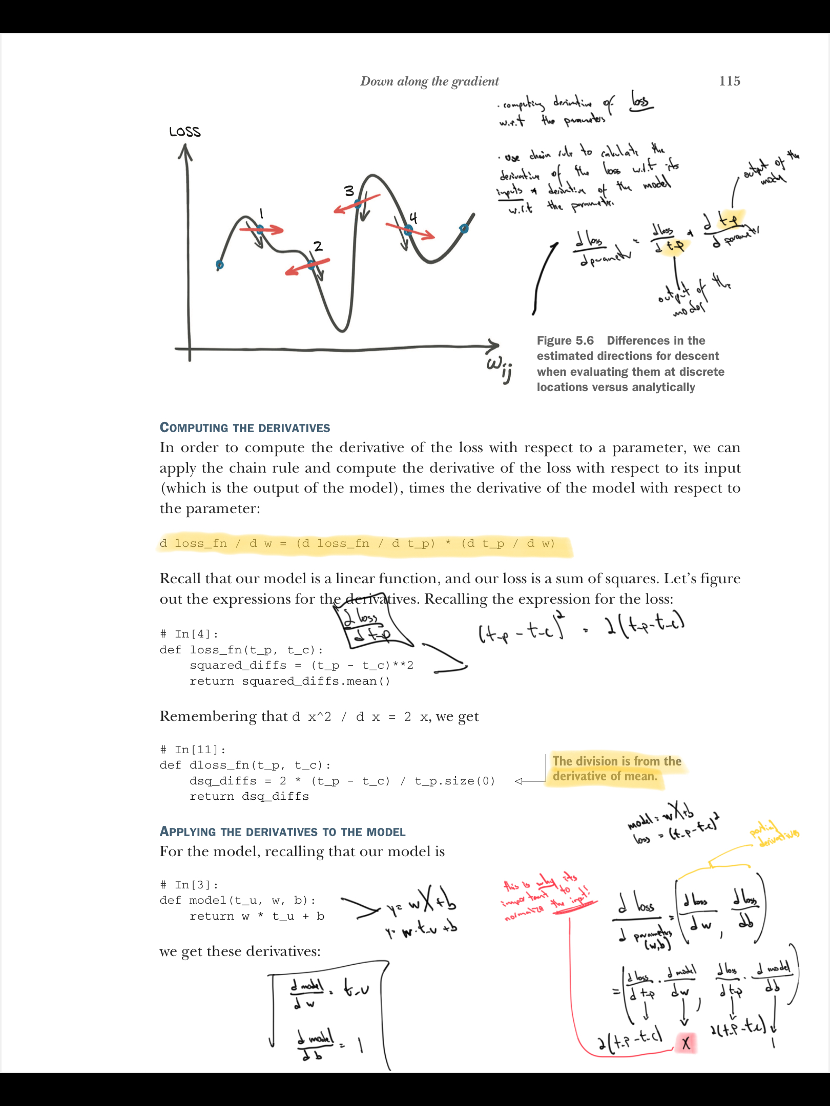
The goal of using derivatives is to guide the model training loop in which directions the parameters of the model need to be updated.
-
We want to optimize the loss function with respect to the weights using gradient descent
From grokking deep learning:
-
“Given a shared error, the network needs to figure out which weights contributed (so they can be adjusted) and which weights did not contribute (so they can be left alone.
-
“Hey, if you want this node to be x amount higher, then each of these previous four nodes needs to be
x*weights_1_2amount higher/lower, because these weights were amplifying the prediction byweights_1_2times.” -p.120
Gradient
The gradient: answers the question: “what is the effect of the weight on the loss function?”

Calculating both direction and amount from error (p.56)
Andrew Trask describes this overall process as predict –> compare –> learn
for iteration in range(20):
    pred = input * weight
    error = (pred - goal_pred) ** 2
    direction_and_amount = (pred - goal_pred) * input
    weight = weight - direction_and_amount
The code above is really the basis of gradient descent. In a single line of code, we are able to calculate both the direction and the amount by which we should make changes to the weight parameters in order to get us a step closer towards some minimum of the loss function. There are some modifications to the above code in practice, inlcuding learning rates, but that really is the main idea.
(pred - goal_pred)
- Example from
micrograd: How are the valuesaandbaffecting g? In other words, what is the derivative of g with respect to a and b?
from micrograd.engine import Value

a = Value(-4.0)
b = Value(2.0)
c = a + b
d = a * b + b**3
c += c + 1
c += 1 + c + (-a)
d += d * 2 + (b + a).relu()
d += 3 * d + (b - a).relu()
e = c - d
f = e**2
g = f / 2.0
g += 10.0 / f
print(f'{g.data:.4f}') # prints 24.7041, the outcome of this forward pass
g.backward()
print(f'{a.grad:.4f}') # prints 138.8338, i.e. the numerical value of dg/da
print(f'{b.grad:.4f}') # prints 645.5773, i.e. the numerical value of dg/db
Happens to be 138, which says, how a affects g through this mathematical expression. If we slightly nudge a and make it slightly larger, it means that g will grow with a slope of 138!. How will g respond if a or b get tweaked a small amount in a positive direction, is what this is answering.
We use this same machinery for nn training. In real rtaintraininging, we use tensors, not scalars.
Recipe
We need to use chain rule to compute the derivative of loss w.r.t to its inputs * derivative of model w.r.t the parameter.
$d_{loss}/d_{parameter} = d_{loss}/d{modelOutput} * d_{modelOutput} / d_{parameter} $
-
Normalizing inputs:
- “The weight and bias live in a differently scaled space. If this is the case, a learning rate that’s large enough to meaningfully ipdate one will be so large as to be usntalble for the other.” –p.119
- By normalizing inputs, the gradients will now be of similar magnitude, as we can use a single learning rate for both parameters.
In PyTorch, the gradient gets calcualted and updated using autograd . “given a forward expression, no matter how nested, PyTorch will automatically provide the gradient of that expression with respect to its input parameters.
Code
loss_rate_of_change_b =
    (loss_fn(model(t_u, w, b + delta), t_c) -    # If you increase b, you get 110 loss for example
    (loss_fn(model(t_u, w, b - delta), t_c) /    # If you decrease b, you get 95 loss for example
    2.0 * delta                                  # For this example the change is positive, so we need to decrease b


b = b - learning_rate * loss_rate_of_change_b
Understanding Backprop
Resources here