## The idea is to build a Vit from scratch, so we'll start with a skeleton of everything we need:
import torch


class ViT(nn.Module):
      def __init__(self, img_size, patch_size, num_hiddens, num_heads, num_classes, depth=6, dropout=0.1):
          super().__init__()
          self.num_patches = (img_size // patch_size) ** 2

          # --- Patch Embedding ---
        #   self.patch_embedding =

          # --- CLS token ---
        #   self.cls_token

          # --- Positional Embedding (+1 for CLS) ---
        #   self.pos_embedding =

          # --- Transformer Encoder ---
          # TODO: stack of transformer blocks goes here

          # --- Classification Head ---
          # TODO: LayerNorm + Linear(num_hiddens, num_classes)

      def forward(self, x):
          batch = x.shape[0]

          # 1. Patch embed: [B, 3, H, W] -> [B, num_patches, num_hiddens]


          # 2. Prepend CLS token: [B, num_patches, D] -> [B, num_patches+1, D]


          # 3. Add positional embeddings


          # 4. Transformer encoder
          # TODO: x = self.transformer(x)

          # 5. Classification: extract CLS token -> head
          # TODO: return self.head(x[:, 0])

return x # placeholder — returns full sequence for nowRe-implement basic ViT from scratch
📚 Resources
Essential Paper: - https://arxiv.org/abs/2010.11929 - Dosovitskiy et al.
Reference Implementations: - https://github.com/lucidrains/vit-pytorch - Clean, minimal implementation - https://github.com/google-research/vision_transformer - Official JAX implementation - https://github.com/huggingface/transformers/blob/main/src/transformers/models/vit/modeling_vit.py
Tutorials & Explainers: - https://jalammar.github.io/illustrated-transformer/ - Jay Alammar - https://www.youtube.com/watch?v=TrdevFK_am4 - https://nlp.seas.harvard.edu/2018/04/03/attention.html
Building Blocks
| Component | Task |
|---|---|
| PatchEmbedding | Patch Embedding class |
| Attention | Have multiple versions |
| FeedForward | Define the MLP block |
| TransformerBlock | Combine attention + FFN + residuals + LayerNorm |
| ViT (full) | Add classification head, add MHA stacking |
| Training loop | Train on CIFAR-10 or MNIST |
youtube link to a good tutorial: https://www.youtube.com/watch?v=7o1jpvapaT0&t=1604s
Intuition for steps:
- Image to patches
- Think of these as the tokens in NLP. Words into tokens and images into patches. Token ids will be the pach indeces.
- Patch embedding
- converts patch index into dense vectors. token embeddings in NLP will be our patch embeddings in ViT.
- Flattened patches (needs to be 1d data vectors) (embedding Layer)
- Add positional embeddings
- Same as in NLP. Give transformer ability to learn location/spatial information.
- Add a
cls_tokenfor classification. Learnable token or vector represent the whole image. This is what is used for classification. - Feed into Transformer Encoder
- Patches and positional info.
- MHA -> Add and Norm -> FeedForward -> Add and Norm.
- Pass into classification head.
Step 1 handle Patch Embedding
this takes an image, and breaks it up into patches.
some implementations do it with einops, others with a convolution.
if the patch size is 14x14, then we can take a convolution and go from 3 channels to hidden_dim (imagine our input is 224x224).
the kernel size is the patch size, effectively giving us patches
import torch
import torch.nn as nn
import torch.nn.functional as F # This gives us the softmax()
import math
class PatchEmbedding(nn.Module):
def __init__(self, img_size, patch_size, num_hiddens):
super().__init__()
self.img_size = img_size
self.patch_size = patch_size
self.num_hiddens = num_hiddens
self.num_patches = int((self.img_size**2) / (self.patch_size**2))
self.conv = nn.Conv2d(in_channels=3,
out_channels = num_hiddens,
kernel_size = patch_size,
stride = patch_size)
def forward(self, x):
x = self.conv(x)
return x# !pip install requestsSome sample data
from torchvision.datasets import FashionMNIST
import torchvision.transforms as transforms
from torch.utils.data import DataLoader
import matplotlib.pyplot as plt

class_names = ['T-shirt/top', 'Trouser', 'Pullover', 'Dress', 'Coat',
                 'Sandal', 'Shirt', 'Sneaker', 'Bag', 'Ankle boot']

train_dataset = FashionMNIST(
      root='./data',
      train=True,
      download=True,
      transform=transforms.ToTensor()
  )

test_dataset = FashionMNIST(
    root='./data',
    train=False,
    download=True,
    transform=transforms.ToTensor()
)

train_loader = DataLoader(train_dataset, batch_size=32, shuffle=True)
test_loader = DataLoader(test_dataset, batch_size=32, shuffle=False)
import matplotlib.pyplot as plt
import torchvision.transforms as transforms
from PIL import Image
import requests
from io import BytesIOurl = "https://ultralytics.com/images/bus.jpg"
img = Image.open(BytesIO(requests.get(url).content)).convert('RGB')
img
transform = transforms.Compose([
      transforms.Resize((224, 224)),
      transforms.ToTensor(),
  ])
img_tensor = transform(img).unsqueeze(0)  # [1, 3, 224, 224]
# Create patch embedding
patch_emb = PatchEmbedding(img_size=224, patch_size=16, num_hiddens=512)
output = patch_emb(img_tensor)
print(output.size())torch.Size([1, 512, 14, 14])So now we have 14 x 14 grid over the entire image of 16x6 patches. The hidden dimension we picked above is 512, so we have a vector of length 512 for each patch.
fig, axes = plt.subplots(1, 3, figsize=(15, 5))

# 1. Original image
axes[0].imshow(img_tensor.squeeze().permute(1, 2, 0))  # [H, W, C]
axes[0].set_title(f'Input: {tuple(img_tensor.shape)}')
axes[0].axis('off')

# 2. Image with patch grid overlay
axes[1].imshow(img_tensor.squeeze().permute(1, 2, 0))
for i in range(0, 224, 16):
    axes[1].axhline(y=i, color='red', linewidth=0.5)
    axes[1].axvline(x=i, color='red', linewidth=0.5)
axes[1].set_title(f'14×14 = 196 patches (16×16 each)')
axes[1].axis('off')

# 3. Output feature map (first 16 channels as a grid)
out_viz = output.squeeze()[:16].detach()  # first 16 of 512 channels
grid = out_viz.reshape(4, 4, 14, 14).permute(0, 2, 1, 3).reshape(56, 56)
axes[2].imshow(grid, cmap='viridis')
axes[2].set_title(f'Output: {tuple(output.shape)}\n(showing 16 of 512 channels)')
axes[2].axis('off')

plt.tight_layout()
plt.show()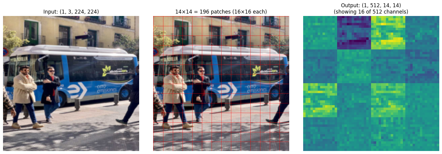
- alternative using einops like
lucidrains:
self.to_patch_embedding = nn.Sequential(
            Rearrange('b c (h p1) (w p2) -> b (h w) (p1 p2 c)', p1 = patch_height, p2 = patch_width),
            nn.LayerNorm(patch_dim),
            nn.Linear(patch_dim, dim),
            nn.LayerNorm(dim),
        )
b = batch_size
c = channels
(h p1) = height
(w p2) is the width
What are some differences in these two implemetations of PatchEmbeddings? Efficiency?
Almost mathematically equivalent, conv2d is more effieicnt. Lucidrains adds LAyerNorm before and after the projectin, which stabilizes training but the two approaches are no longer equivalent. I once heard Daniel Han say “just add LAyerNorm” everywhere, so maybe we stick with that.
Conv2d approach bakes in an assumption that kernel_size = stride =patch_size which makes it harder to operate on non-square images?
14*14 # <- this is the number of patches we have, we now need to flatten them196output_flat = output.flatten(2)
print(output_flat.size())
output_flat_transposed = output_flat.transpose(1,2)
print(output_flat_transposed.size()) # now this is ready to gotorch.Size([1, 512, 196])
torch.Size([1, 196, 512])Positional Embeddings
For each vector of size 512 (one per patch) we add positional encoding.
Why do we need positional embeddings in the first place? The self-attentnion mechanism is permutation invariant. So if we were to randomly shuffle our ptaches from the aboce PAtchEmbedding layer, the attention mechanism would output the same just in a different order.
So we just add a self.pos_embedding. This is one vector per position of the patch. It will look something like self.pos_embedding = nn.Parameter(torch.randn(1), num_patches + 1, hiddem_dim)
Model will learn these during training. So position 0 means top-left and position 13 means end of first row. This is from the orginal ViT paper implementation.
# use sin/cos waves ar different frequencies. Each dimension gets a different frequency, so each position gets its own.
def sinusoidal_positional_encoding(num_positions, dim):
      """
      PE(pos, 2i)   = sin(pos / 10000^(2i/dim))
      PE(pos, 2i+1) = cos(pos / 10000^(2i/dim))
      """
      position = torch.arange(num_positions).unsqueeze(1).float()  # [num_positions, 1]
      div_term = torch.exp(torch.arange(0, dim, 2).float() * -(math.log(10000.0) / dim))  # [dim/2]

      pe = torch.zeros(num_positions, dim)
      pe[:, 0::2] = torch.sin(position * div_term)  # even indices
      pe[:, 1::2] = torch.cos(position * div_term)  # odd indices
      return pe  # [num_positions, dim]
import matplotlib.pyplot as plt
import math
def sinusoidal_positional_encoding(num_positions, dim):
position = torch.arange(num_positions).unsqueeze(1).float()
div_term = torch.exp(torch.arange(0, dim, 2).float() * -(math.log(10000.0) / dim))
pe = torch.zeros(num_positions, dim)
pe[:, 0::2] = torch.sin(position * div_term)
pe[:, 1::2] = torch.cos(position * div_term)
return pe
pe = sinusoidal_positional_encoding(197, 512) # 196 patches + 1 CLS
fig, axes = plt.subplots(1, 2, figsize=(16, 5))
# Left: full heatmap
im = axes[0].imshow(pe.numpy(), aspect='auto', cmap='RdBu')
axes[0].set_xlabel('Embedding dimension')
axes[0].set_ylabel('Patch position')
axes[0].set_title('Sinusoidal Positional Encoding (197 positions × 512 dims)')
plt.colorbar(im, ax=axes[0])
# Right: show individual dimensions as waves
for d in [0, 1, 10, 50, 100, 255]:
axes[1].plot(pe[:, d].numpy(), label=f'dim {d}')
axes[1].set_xlabel('Patch position')
axes[1].set_ylabel('Encoding value')
axes[1].set_title('Individual dimensions — low dims = high freq, high dims = low freq')
axes[1].legend()
plt.tight_layout()
plt.show()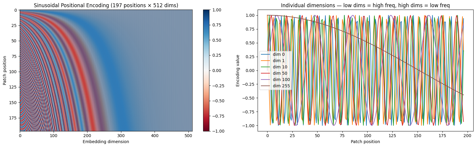
each row is one patch position. (0-196). Each column is one dimension of the embedding vector.
Int he lower dimensions, there are rapid alternating stripes. these are high frequency sin/cos waves that change quickly between adjacent positions. Help model distingiuish between neighboring patches.
In the higher dimensions, there are wide slow changing bands. these help the model distiniguish ebtween patches that are far apart.
every position gets a unique combination of high-frequence and low-frequency signals.
Transformer Blocks
## FeedForward, just linear layers with GELU and some dropout
class FeedForward(nn.Module):
    def __init__(self, dim, hidden_dim, dropout = .1):
        super().__init__()
        self.net = nn.Sequential(
            nn.Linear(dim, hidden_dim),
            nn.GELU(),
            nn.Dropout(dropout),
            nn.Linear(hidden_dim, dim),
            nn.Dropout(dropout)
        )

    def forward(self, x):
        return self.net(x)
input (512) → Linear → GELU → Linear → output (512)
512 → 2048 → 2048 → 512
- Attention in the transformer block tells us which patches we should look at (context)
- The FeedForward layer tells the model what to actually do with that context and the other patches.
### Single Attention HEad
class AttentionHead(nn.Module):
    def __init__(self, dim, head_dim, dropout = .1):
        super().__init__()
        self.scale  =  head_dim ** -0.5
        self.q = nn.Linear(dim, head_dim, bias = False)
        self.k = nn.Linear(dim, head_dim, bias = False)
        self.v = nn.Linear(dim, head_dim, bias = False)
        self.dropout = nn.Dropout(dropout)

    def forward(self, x):
        q, k, v = self.q(x), self.k(x), self.v(x)
        attn = torch.matmul(q, k.transpose(-1, -2)) * self.scale
        attn = F.softmax(attn, dim =-1)
        attn = self.dropout(attn)
        out = torch.matmul(attn, v)
        return out
There are 3 projections of our data, Q,K,V. Each one of them kind of asks a specific question.
Q asks, what am I looking for? SO this patch needs something, what is it?
K: asks what do I contain?
V: says, here is what I actually contain. This is what is passed along if a patch is actually selected as context.
The attention score from the paper is Q@K^T. This is just the dot product of every query and key. This tells us how much should patch i attend to path j in a NxN matrix. If the dor product is hight and same direction, then its high value.
We use self.scale because without the dot products grow in magniture as head_dim gets bigger. This keeps the variance closer to one and softmax remains useful.
Softmax: turn values into weights or a porbability distribution.
attn @ V:
out = torch.matmul(attn, v)now, each patch’s output is a weighted combination of all patches’ values using the attention weights. So for example path i will have mostly values from whichever patches it attended to.
class MultiHeadAttention(nn.Module):
    def __init__(self, dim, num_heads, dropout=0.1):
        super().__init__()
        assert dim % num_heads == 0, "dim must be divisible by num_heads"
        self.head_dim =  dim // num_heads
        self.num_heads = num_heads
        self.heads =  nn.ModuleList([
            AttentionHead(dim, self.head_dim, dropout) for j in range(num_heads)
        ])
        self.proj = nn.Linear(dim, dim)
        self.dropout = nn.Dropout(dropout)

    def forward(self, x):
        head_outputs = [head(x) for head in self.heads]
        out = torch.cat(head_outputs, dim = -1)
        out = self.proj(out)
        out = self.dropout(out)
        return out
Multi head is now just several attention heads stacked. Why? We split the input dimensions into several heads. Each head gets its own Q,K,V projections and lears its own attentnion weights independently.
Each head sees the full input but projects it down. This means that we get diverse attention patterns from each head, but since we split the input, its the same computational cost.
In the forward pass, we run all heads with the same full input [B, 197, 512]. Each head will project it down to [B, 197, 64] So we get 8 of those, one for each head.
We concatenate all of them along the last dimensino and we have a single tensor with info gathered from all 8 heads.
The self.proj then mixes all the independent stacks across. It lets the model figure out how to combine all the heads inputs in a way that makes sense for the task.
class TransformerBlock(nn.Module):
    def __init__(self, dim, num_heads, mlp_dim, dropout=0.1):
        super().__init__()
        self.norm1 = nn.LayerNorm(dim)
        self.attn = MultiHeadAttention(dim, num_heads, dropout)
        self.norm2 = nn.LayerNorm(dim)
        self.ffn = FeedForward(dim, mlp_dim, dropout)

    def forward(self, x):
        # Pre-norm style (what ViT uses, unlike original transformer)
        x = x + self.attn(self.norm1(x))
        x = x + self.ffn(self.norm2(x))
        return x
TransformerBlock is the core repeating unit. IT has 2 simple sub-steps.
step1: self.norm, self.attn, and residual connection.
step2: feed forward. this processes each patch independently and then adds it back to residuals.
The transformer block does:
  Input
    │
    ├──── LayerNorm → MultiHeadAttention ────┐
    │                                         │
    └──────────── + (residual) ◄─────────────┘
    │
    ├──── LayerNorm → FeedForward ───────────┐
    │                                         │
    └──────────── + (residual) ◄─────────────┘
    │
  Output
class TransformerEncoder(nn.Module):
def __init__(self, dim, depth, num_heads, mlp_dim, dropout=0.1):
super().__init__()
self.layers = nn.ModuleList([
TransformerBlock(dim, num_heads, mlp_dim, dropout)
for _ in range(depth)
])
self.norm = nn.LayerNorm(dim) # final norm after all blocks
def forward(self, x):
for block in self.layers:
x = block(x)
return self.norm(x)the last step is the full encoder.
Stacks N transformer blocks in a squence. This is similar to how CNNs stack layers, so early blocks will learn low-level things like local features, textures, edges and later blocks learn more high level information like semantic meaning.
encoder = TransformerEncoder(dim=512, depth=6, num_heads=8, mlp_dim=2048, dropout=0.1)
dummy = torch.randn(16, 197, 512)  # (batch, num_patches+1, hidden_dim)
out = encoder(dummy)
print(out.shape)  # should be [16, 197, 512]
print(f"Parameters: {sum(p.numel() for p in encoder.parameters()):,}")
torch.Size([16, 197, 512])
Parameters: 18,906,112class ClassificationHead(nn.Module):
def __init__(self, hidden_dim, num_classes):
super().__init__()
self.norm = nn.LayerNorm(hidden_dim)
self.linear = nn.Linear(hidden_dim, num_classes)
def forward(self, x):
cls_t = x[:, 0]
out = self.norm(cls_t)
out = self.linear(out)
return out
class ViT(nn.Module):
      def __init__(self, img_size, patch_size, num_hiddens, num_heads, num_classes, depth=6, dropout=0.1):
          super().__init__()
          self.num_patches = (img_size // patch_size) ** 2

          # --- Patch Embedding ---
          self.patch_embedding = PatchEmbedding(img_size, patch_size, num_hiddens)

          # --- CLS token ---
          self.cls_token = nn.Parameter(torch.randn(1, 1, num_hiddens))

          # --- Positional Embedding (+1 for CLS) ---
          self.pos_embedding = nn.Parameter(torch.randn(1, self.num_patches + 1, num_hiddens))

          # --- Transformer Encoder ---
          self.encoder = TransformerEncoder(num_hiddens, depth, num_heads,  mlp_dim=num_hiddens*4)

          # --- Classification Head ---
          self.classification_head = ClassificationHead(num_hiddens, num_classes)

      def forward(self, x):
          batch = x.shape[0]

          # 1. Patch embed: [B, 3, H, W] -> [B, num_patches, num_hiddens]
          patches = self.patch_embedding(x)
          patches = patches.flatten(2).transpose(1, 2)

          # 2. Prepend CLS token: [B, num_patches, D] -> [B, num_patches+1, D]
          cls_tokens = self.cls_token.expand(batch, -1, -1)
          x = torch.cat((cls_tokens, patches), dim=1)

          # 3. Add positional embeddings
          x = x + self.pos_embedding

          # 4. Transformer encoder
          x = self.encoder(x)

          # 5. Classification: extract CLS token -> head
          x = self.classification_head(x)

          return x  # placeholder — returns full sequence for now
Lets test it on FashionMNIST
transform = transforms.Compose([
      transforms.Resize((56, 56)),
      transforms.Grayscale(num_output_channels=3),  # repeat grayscale to 3 channels
      transforms.ToTensor(),
  ])

train_dataset = FashionMNIST(root='./data', train=True, download=True, transform=transform)
test_dataset = FashionMNIST(root='./data', train=False, download=True, transform=transform)

train_loader = DataLoader(train_dataset, batch_size=32, shuffle=True)
test_loader = DataLoader(test_dataset, batch_size=32, shuffle=False)
device = torch.device('cuda' if torch.cuda.is_available() else 'mps' if torch.backends.mps.is_available() else 'cpu')
print(f"Using: {device}")Using: mpsmodel = ViT(
img_size=56, patch_size=7, num_hiddens=256,
num_heads=8, num_classes=10, depth=2, dropout=0.1
).to(device)optimizer = torch.optim.Adam(model.parameters(), lr=3e-4)
criterion = nn.CrossEntropyLoss()
for epoch in range(5):
model.train()
total_loss, correct, total = 0, 0, 0
for images, labels in train_loader:
images, labels = images.to(device), labels.to(device)
logits = model(images)
loss = criterion(logits, labels)
optimizer.zero_grad()
loss.backward()
optimizer.step()
total_loss += loss.item()
correct += (logits.argmax(dim=-1) == labels).sum().item()
total += labels.size(0)
print(f"Epoch {epoch+1} | Loss: {total_loss/len(train_loader):.4f} | Acc: {correct/total:.4f}")Epoch 1 | Loss: 0.6208 | Acc: 0.7683
Epoch 2 | Loss: 0.4294 | Acc: 0.8407
Epoch 3 | Loss: 0.3818 | Acc: 0.8573
Epoch 4 | Loss: 0.3576 | Acc: 0.8671
Epoch 5 | Loss: 0.3407 | Acc: 0.8718model.eval()
correct, total = 0, 0
with torch.no_grad():
for images, labels in test_loader:
images, labels = images.to(device), labels.to(device)
logits = model(images)
correct += (logits.argmax(dim=-1) == labels).sum().item()
total += labels.size(0)
print(f"Test Accuracy: {correct/total:.4f}")Test Accuracy: 0.8721