# TODO
# 1. load 100 MNIST images of one digit
import torch
from torch.utils.data import DataLoader, Subset
from torchvision import datasets, transforms
import matplotlib.pyplot as plt
# Load MNIST (downloads ~10MB on first run)
transform = transforms.ToTensor()
dataset = datasets.MNIST(root='./data', train=True, download=True, transform=transform)

# Take just the first 100 samples
subset = Subset(dataset, range(100))
loader = DataLoader(subset, batch_size=100, shuffle=False)Phase 1 / Week 1 — Representation Learning: Theory & Foundations
Anchor question for Module 3: what does a good representation look like, and how do we know we’ve learned one without labels?
This week’s reading: - Bengio, Courville, Vincent — Representation Learning: A Review and New Perspectives (2013) — https://arxiv.org/abs/1206.5538 - Yann LeCun — Cake analogy + Energy-Based SSL / JEPA talks (e.g. NeurIPS 2016 keynote, AAAI 2020, A Path Towards Autonomous Machine Intelligence position paper, 2022)
What you should be able to do by the end of the week: 1. State, in one sentence each, the ~10 priors Bengio argues a good representation should respect. 2. Explain the difference between invariance and equivariance with a concrete image example. 3. Argue why pixel-space reconstruction is a weak SSL signal (LeCun’s framing — this motivates JEPA later). 4. Reproduce LeCun’s cake analogy from memory, and explain what changed between his 2016 and 2022 versions of it. 5. List 2–3 concrete failure modes of joint-embedding SSL (representation collapse) that any of the methods in Phases 2–3 must avoid.
Learning Representations
Instead of learning f(x) -> y we can learn a representation g: X -> Z and then learn the classifier/predictor f: Z->Y on top of it.
Goal: learn only one/few representations for each domain, then learn simple predictors for different tasks.
Learning g should need no.less different supervision, so w can use more data.
“Ai must […] learn to identify and disentangle the underlying explanatory factors hidden in the observed milieu of low-level sensory data.”
Explanatory factors / factors of variation
- observed data is a causal result of underlying factors, Variations in these explain the variation in the data.
- example: factors of images –> object depicted, rotation, lighting, etc..
- We want to recover the underlying factors.
Bengio : the manifold hypothesis
What is a manifold? Its a set that locally looks like a flat Euclidean space, even though globally it can curve and twist. For example, the earth is an example of a manifold used. If you stand anywhere in the earth it looks flat, but the whole thing is in 3D space.
An n-dimensional manifold M sitting inside R^N is a subset where around every point, you can find a small patch that is smoothly equivalent to a piece of R^N.
The hypothesis: A 224x224x3 image is a point in a universe of R^150k. The majority of the points in an image though are noise. So if we step into the image in a random location, your neighborhood looks like static and probably similar. Natural images occupy a much-lower dimensional subset of the pixel space.
For example, in the MNIST dataset most of the signal in what digit is handwritten is localized in a small subset of the image. Meaning we can probably find a lower-dimensional representation of that set.
The encoder will generally be a map that tries to unfold the data manifold. So for example in V-jepa, trying to predict masked patches forces the model to learn variations of the manifold. So exactly where the semantic signal lives.
What is a good representation?
- captures the posterior distribution of the underlying explanatory factors.
- one that is useful as input to a supervised predictor.
Bengio — the full list of generic priors
Bengio §3 enumerates priors a good representation should encode. You have smoothness, less-supervised, and a version of coherence/invariance above. Below are the rest — fill each one in your own words as you read, with a concrete image/video example where possible.
Convention used below:
prior name — one-sentence definition. Concrete example. Why it matters for SSL.
1. Smoothness
Why is smoothness alone not enough for high-dimensional data? (Hint: curse of dimensionality — local generalization buys you nothing in a space the size of natural images.)
Your note on the curse-of-dim argument:
Basically notes that is x is similar to y, then f(x) must also be similar to f(y). Why curse-of-dimensionality? Most of the linear algorithms that would satisfy smoothness would only exploit the principle of local generalization. So this means they would or could only generalize to nearby points. So once youve seen training points, you can answer queries at nearby points by interpolating. To use a smoothness prior, every test point must have at least one training point within some neighborhood radius, r. How many training points do you need to cover that in d dimensions?
So one question i have is why cant you just pick the closest training point to a query, why do we need radius r? The answer is that in very high dimensions like natural images, the average nearest neighbor distance is roughly half the diameter of the entire space away, so this is basically a random set of points. Theres no meaningful sense in the word ‘near’ anymore in high dimensions. The nearest training point in this case is not meaningfully more similar that then farthest. So smoothness in pixel space gives you no real signal. Once you learn a good representation model that has more that just a smoothness prior, you get “Suddenly 1-NN works again. This is exactly the kNN probe that DINOv2 / V-JEPA / etc. report as a headline number —”kNN @ ImageNet-1k” in your Phase 5 benchmark table. The fact that kNN works at all on top of an SSL feature is the proof that the encoder has put the manifold somewhere the smoothness prior can finally do its job.”
2. Multiple explanatory factors / distributed representations
One-hot vs distributed: why does a distributed code give exponentially more expressive power for the same number of parameters?
Definition:
** the world factorizes, and learning the factors lets you generalize combinatorially rather than memorize**
The paper claims that the world is generated by a small set of underlying factors (object identity, pose, lighting, viewpoint, background …) and that observations are the result of those factors combining. The critical term hes using is generalize. What you learn about how one factor works should transfer across all settings of the other factors.
The data generating distributions is generated by by different underlying factors. For the most part what one learns about one factor generalizes in many configurations of the other factors. This assumption is behind the idea of distributed representations.
- representations are expressive, meaning that a reasonably-sized learned representation can capture a huge number of possible input configurations.
This is one of the technical core of the whole paper
- distributed representations buy you and exponential number of distinct input regions for the price of a linear number of parameters.
Distributed representations:
Example (image):
Say you are working on a face/identity classifier. You re experimenting with what rotation does to faces. You see person A rotated through many angles. Now person B walks in (youve never seen this person rotated before ). The claim is: if your model learned rotation as its own factor, you already know that person B looks like rotated! You dont have to explicitly relearn the rotation of every identity you see.
Faces, three features: “glasses”, “beard”, “smiling”.
One-hot / local approach. You’d need one anchor per person-state: Alice-glasses-beard-smiling, Alice-glasses-beard-frown, Alice-glasses-clean-smiling, … For one person across the 8 combinations of three binary attributes, that’s 8 anchors.
For 100 people: The model has to individually represent every cell of the combinatorial grid.
Distributed approach. Three feature detectors, total. Each one is a hyperplane that responds to its attribute regardless of who is wearing it. The representation of any input is (g, b, s) ∈ {0,1}^3, picking out one of 8 cells. With three parameters you’ve described 8 cells for any person. Add 4 more features (identity-related) and you can now describe 100 people × 8 attributes = 800 cells using just 7 features instead of 800 anchors. The exponential blow-up of the combinatorial grid is implicit in the distributed code — you never have to enumerate it.
Why it matters for SSL:
If there are k factors and each can take a set of values, the number of possible observations grown combinatorially. A representation encodes the Factors themselves and can describe any combination, including unseen combinations. Thats the main thing that lets representation learning generalize beyond the training set. Hence the name distributed representations.
The models we use now like SimCLR, DINO, MAE, VJEPA all produce distributed representations. If we produce a [1x768] embedding vector, those are not 768 independent local anchors, they are 768 features, jointly finding space in feature space to a combinatorial number of cells.
Other thoughts
When DINOv2 (or any modern SSL model) reports “kNN @ ImageNet-1k” or “linear probe @ ImageNet-1k,” the headline is precisely: the 768-D code is so well-structured that a trivial reader (Euclidean distance / linear weights) can extract any class. No fancy head needed. That works because the code is distributed.
3. Hierarchical organization / depth
Composition of simple features → complex features. Why does this map onto deep nets specifically?
Definition:
There are advantages to learning good representations. 1. deep architectures promote the re-use of features 2. deep architectures can potentially lead to progressively more abstract features at higher layers of representations.
What is feature re-use?
This is essentially the power of distributed representations. We described above that doing one-hot encodings of features is less powerful than getting a vector representation for that feature that can easily combined with other features.
What is abstraction and invariance?
Deep representations can carry more abstract concepts that clustering for example. Cluster membership is one anchor, but with good representations you can have more abstract groupings of samples. Abstract concepts can be more invariant to local changes of the input. If we think about face rotation for example, if our representation is capturing general likeness by representing attributes of a face, it should be invariant of rotations. Learning these sorts of invariant features has been a long-standing goal in pattern recognition.
- Lower layers: high resolution, selective (a unit fires on a specific edge at a specific location), not invariant (shift the image, the unit shifts).
- Higher layers: pooled across larger receptive fields, invariant (the “face” detector doesn’t care exactly where the eyes are), but less selective to local detail.
So deeper ≠ “just more abstract.” Deeper = “pooled more, so invariant to more transformations, at the cost of throwing away local detail you no longer need.”
Example (image):
The canonical one (Zeiler & Fergus 2014, “Visualizing and Understanding Convolutional Networks”) makes the hierarchy literal:
- Layer 1: edges, color blobs.
- Layer 2: corners, simple textures (combinations of layer-1 edges).
- Layer 3: object parts — wheels, eyes, fur patterns (combinations of layer-2 textures).
- Layer 4+: whole objects — faces, cars, dogs. Each layer is a combination of the previous level’s features. Thats the picture of compositional feature re-use.
Why it matters for SSL:
- we established why distributed features is important to ssl.
- Abstraction and invariance follow that logic somewhat which is we want representations that are invariant to small input changes like rotation, in other words they capture the semantic meaning of the input and dont change much by local changes.
- predicting in representation space (as v-jepa does) is only useful is the representation space is high in the hierarchy. Predicting masked-region pixels like MAE, burns capacity on low-level texture. So depth drives abstraction.
4. Semi-supervised learning
Restate in Bengio’s exact framing: when is P(X) informative about P(Y|X)? When is it not?
Your note:
In ML we usually set up supervised learning as getting features from X to learn y. The task is P(Y|X). In the paper, they claim that if we learn good representations of P(X) then they will be useful when learning P(Y|X). P(X) helps in learning P(Y|X) because the underlying factors of variation that generate X tend to be the same ones that predict Y.
- If we can learn a representation that captures the underlying factors from unlabeled data, just X to learn Z, then
P(Y|Z)is easy to learn from less labels. This is the prior that justifies SSL’s existence!!
6. Manifold hypothesis
Natural data concentrates near a low-dimensional manifold embedded in a high-dim ambient space.
Definition:
The manifold hypothesis states that natural data concentrates on a low-dimensional manifold inside the high-dimensional pixel space, where the intrinsic dimensions of the manifold correspond to the underlying factors of variation. . The hypothesis: A 224x224x3 image is a point in a universe of R^150k. The majority of the points in an image though are noise. So if we step into the image in a random location, your neighborhood looks like static and probably similar. If you sampled a random vector from R^150k, the result would look like static — natural-looking images occupy a vanishingly small, curved sub-region of that space.
Example — sketch (or describe) the manifold of MNIST 3s under rotation:
MNIST images live in R^784. But the set of valid handwritten digits is a vanishingly small, curved subset of that 784-D space — most 784-D vectors look like static, not digits. The “manifold of MNIST digits” is the surface this small subset occupies.
If we take an image from MNIST as rotate it from 0-360 degrees in 1 degree steps: * each rotations gives a different 784-D vector of pixels. * if we wanted to find the angle of rotation, we would need only one parameter while the space lives in 784-D. * So intrinsic dimension of the set of vectors is 1D, just the rotation * the ambient dimension is 784.
If we then just varied stroke width on top of the rotation then the set is a 2D manifold. If we add writer style, we go to 3D. So the intrinsic dimension grows by one if we add one factor of variation, not with the pixel count of the images.
Why it matters for SSL (connect to contrastive geometry — Phase 2):
…
7. Natural clustering
Class-conditional density tends to concentrate, with low-density regions between classes.
Definition:
Separate manifolds tend to contain separate categories. Local variation in a manifold are small changes within a category. Jumping from region of one class to another involves travelling through low density regions.
- in fact, class boundaries lie in the valleys of
P(X). - natural clustering states that the surface of the low-dimensional space our data lives in has clumps. Each class is its own connected region, separated from other by low-density gaps.
Where you’ll see this used explicitly (hint: SwAV, DeepCluster, DINO centering):
DINO centering is used in DINO as a way to prevent collapse (keeping the softmax from becoming uniform).
Why it matters for SSL: The natural clustering prior is what justifies treating :grouping similar inputs together” as a useful training signal at all. This is where contrastive learning can kick in directly with this prior, along with smoothness. If P(X) did not actually cluster by category then clustering based SSL would not work. We would be trying to group things with uncorrelated semantics! This prior is the main assumption that lets unsupervised clustering recover the true semantic categories we might be after.
8. Temporal & spatial coherence (slow features)
Consecutive video frames share most factors; nearby image patches share most factors.
Definition:
We expect representations to change slightly given a small variation of the input. Whether that is a consecutive frames in a video or neighboring patches of input. Temporal coherence can be expressed simply as the squared difference between feature values at times t and t+1.
- The reason this prior is so productive is that the temporal coherence makes time itself the free label which we can exploit to learn good representations. Consecutive frames themselves become the free label.
Connection to a method you’ll implement (CVRL / V-JEPA — Phase 4):
In DINO and other methods we expect small variations (crops) of the input to produce small or no variations in the representations if they are learning semantics. In MAE for example, we also use spatial coherence to learn masked patches given the unmasked context. We can exploit this measure to make sure we get good representations. In video like VideoMAE and VJEPA, we exploit both temporal and spatial coherence by masking out entire tubes of input. In other words, find features that are slow-changing across consecutive frames, but not collapsed to zero. <- Every video SSL method used this prior. When a factor is multi-dimensional, its components vary in a coordinated way.
Slow Feature Analysis (Wiskott & Sejnowski 2002) is the formal anchor: find features that are slow-changing across consecutive frames, but not collapsed to zero. Every video SSL method since is a variation on this .
CVRL contrastive over time, VideoMAE / V-JEPA via tube masking. The prior makes time itself the free supervision signal, which is why video SSL can scale to YouTube-volume unlabeled data.
9. Sparsity
Most factors are irrelevant for any given observation — only a few are ‘on’.
Definition:
Given the above, we expect extracted features to be insensitive to small variations of the input. When you look at a cat picture the relevant factors we need to classify are things like is-cat, is-indoors, is-orange, is-furry. But for natural images, hundreds of other factors are defined in the representation space, things like is-galaxy, is-underwater, is-shiny. For this particular image, all of those would be close to 0 (sparse). The world (universe distribution) generates outputs that combine a few of those factors at a time, not all. Representations should reflect that structure.
- Methods will add L1 on the loss to push most units to 0. Think of this as Lasso regression to push coefficients to exactly 0.
- ReLus naturally produce some sparsity.
- bias also can push things down.
- most modern SSL methods do not enforce sparsity harshly, instead they can use general direction of activations as signal, more negative more positive etc..
Tension with smoothness — when do these priors fight each other?
Putting hard limits on sparsity and making things exactly zero can break smoothness. If you have a single unit h(x) over a scalar input x ∈ [-1, 1]. Lets say this unit’s job is to detect the presence of is-furry. It should be 0 when that factor is absent and higher than zero when its present.
- if we enforce maximal sparsity (i.e
h(x) = 1 if x > 0.6 else 0) it will be sparse, but it wont be smooth. an input of x = 0.6 it will jump. So tiny inputs at the input will make step changes and therefore not be smooth. - if we enforce maximal smoothness (i.e
h(x) = sigmoid(10·(x - 0.6))) it will be smooth, but it wont be sparse. Even if we are far away from the threshold, it wont be exactly 0. Inputs will always activate a tiny bit. - Say we use ReLu though,
h(x) = max(0, x - 0.6), it will be 0 at anything less than 0.6. It will be smooth since there is no step-jump at the threshold. BUT it wont be differentiable at exactly the threshold.
In geometry terms, a purely smooth representation will be continuous, no tearing. A purely sparse representation with have partitions in the input space. Partition boundaries are where two different subset will meet and that will change discretely.
Modern SSL methods tackling this tension
- Soft activations like GELU, SiLU, Swish. these are the smooth versions of ReLU without the kink. It will enforce near-sparsity and is differentiable.
- L2 instead of L1. So Ridge instead of Lasso, we penalize the sum of squared coefficients and it will shrink coefficients toward zero, but not exactly zero.
10. Simplicity of factor dependencies
In a good representation, the factors should depend on each other in simple ways — ideally linearly.
Definition:
in a good representation Z the map from the representation to any downstream quantity (label Y or another factor F) should be simple and ideally linear.
The encoder is actually being tasked with untangling the world. By the time data reaches
Z, downstream models should be able to recover the factors of variation with a trivial function.interestingly Locatello et al. 2019 proved that unsupervised disentanglement is fundamentally impossible without inductive biases. There’s no way for an encoder, given only unlabeled data, to know that your axis-of-interest should be coordinate 437.
Why this is the assumption behind linear probing as an SSL eval (forward-link to Phase 5):
This is important because lots of representation learning is evluated on its ability to do tasks well with a simple linear probe. The idea is that the representations are alreay so good that a simple linear probe will get good results on varied tasks.
Summary of 10 priors
- smoothness: the encoder is a continuous function. Every SSL method assumes this.
- Distributed representations: N units encode up to 2^N configurations via parameter reuse, not anchor lookup.
- Hierarchy/ depth: features compose. High level features are functions of lower-level features. Adds another exponential gain on top of distributed representations.
- semi-supervised learning:
P(X)is informative aboutP(Y|X)because they share underlying factors. This is the main justification for SSL! - shared factors across tasks: The same factors that can predict one Y we care about can also predict Y_2, Y_3 etc… One backbone -> many heads. Proven with DINOv2, SAM, DETR pretraining, and V-JEPA multi-task evaluations.
- manifold hypothesis: data concentrated in a low-dimensional manifold in high-dimension input ambient space. The intrinsic dimension of the manifold is the number of underlying factors. This is why KNN works on SSL features but not on raw pixels.
- natural clustering: the manifold is clumpy. Classes occupy connected regions separated by low-density valleys. This justifies contrastive learning and grouping similar things as a training signal.
- temporal and spatial coherence (slow features): nearby frames in videos and nearby patches in images share most underlying factors. Factors will change slowly over time and space. This gives is another free supervision signal. Anchors are SFA, CVRL, VideoMAE, V-JEPA.
- sparsity: Each observation involves only a few of the many possible underlying factors. Most representation dimensions should be 0 or close to 0. Not strictly enforced in modern SSL.
- simplicity of factor dependencies: Factors should be recoverable from the representation by a simple (ideally linear function).
These priors are not independent from one another. They stack on top of each other and nest.
The world’s data lives on a low-dim, clumpy, coherent manifold whose intrinsic coordinates are generative factors. A good encoder maps observations onto this manifold by composing simple features into complex ones (depth) while reusing parameters across inputs (distributed reps), so that downstream tasks (which depend on the same factors ) can be solved with trivial linear readouts on top.
Remember these priors as we go on in the course:
- In Phase 2 we start contrastive learnings. priors 1, 6 and 8 emerge when we visit augmentation invariance and alignment.
- In Phase 3 when we visit distillation, we need priors 3 and 10 to understand depth and linear probing ability.
- In Phase 4 for video we need prior 8.
- In Phase 5 for evaluations we use prior 6 to use KNN probing, prior 10 for linear probes and prior 5 to test for transfer/multi-tasks, and prior 7 for a clustering evaluation.
Disentanglement — a closer look
Bengio’s strongest claim: a representation is disentangled if the latent units align with the true underlying factors (object identity, pose, lighting, …) such that changing one factor changes one (or few) units.
Q1. Write down a definition of disentanglement that doesn’t presuppose access to the true factors. (Why is this hard?)
Disentangled representations match exactly one factor to one dimension of the representation (or a small disjoint group of representations). Intervening on one factor changes only its assigned subset, and each factor is recoverable from that subset alone.
Disentanglement is not about how much information the repersentation contains, its about how the information is organized along the coordinate axes.
Q2. What’s the difference between disentanglement and invariance? A representation that’s invariant to lighting is, in a sense, throwing lighting away. A disentangled one separates it. When do you want which?
In inavariance, we want repreentations that do not change with small changes to inputs. In other words, we want out reps to be able to throw away information about factors changing when those factors are uninformative. For example a rotation or a color jitter is un-informative to a classification task. But dinsentglement refers to preserving information about factors like shadows, which we want our features too show and keep that information, but its ultimately a factor that should not change the classification of an image.
Q3. Locatello et al. 2019 (Challenging Common Assumptions in Disentanglement) showed that unsupervised disentanglement is fundamentally impossible without inductive biases. Skim the abstract — what’s the impossibility result?
Using disentanglement metrics like BetaVAE score: * can a simple classifier predict which factor was held constant given a pair of inputs that share one factor? * sample 2 inputs with one factor matched that tke absolute difference of their latent, train a low-capacity linear classifier to predict the held-fixed factor. * FactorVAE Score: * measures for each fixed factor, find the latent dimension with the smallest normalized variance across the batch –> tries to find “this is the dim that encodes this factor” * MIG - mutital information gap: * for each factor, the gap between the latent dim with the highest mututal information about f_i and the second highest. * DCI - disentaglement/completenedd.informativeness * measure three spearate scores from feture-importance weights of a predictor trained to map z-> f.
they show that well-disentangled models seemingly cannot be identified without access to ground-truth labels even if they are allowed to transfer hyper-parameters across data sets. Furthermore, increased disentangledness does not seem to lead to a decreased sample cmplexitiy of learning for downstream tasks. This basically knocks the windo out of disentanglement-as-objective research.
Invariance vs. equivariance — make this precise
The distinction matters a lot for detection/segmentation (Module 2) and for video SSL (Phase 4).
Let T be a transformation on the input (e.g. translation) and g the encoder.
- Invariant:
g(T x) = g(x)— the rep doesn’t move when the input moves. - Equivariant:
g(T x) = T' g(x)— the rep moves in a predictable way (someT') when the input moves.
Q1. For a classification head, do you want translation invariance or equivariance in the backbone? Why?
You want invariance in the final classification outputs since you care about just what is in the image. But in the backbone, you might want or cant control if its invariant or not.
convnets actually might be equivariant in the first layers, since shofts in put shift the outputs. At the end with the global average ppoling, you should get invariance.
Q2. For a detection head (DETR — you’ll build this in Module 2), which do you want?
For a detection head, you want equivariance. if the input moves slightly to the left, you want to map that in a predictable way.
- DETR works on a 2D grid of feature tokens, each has a positional embedding encoding its spatial location on the grid.
- If the input shifts, the backbone should be shifting in the grid in the same way (predictable)
- The queries in the DETR decoder can then localize the objects using the positional encodings attached to each token.
Q3. Contrastive SSL with random crops forces approximate invariance to crop position. Is that always desirable? When does it hurt?
In DINO for example, student model gets a cropped or distorted version of the input while the teacher gets a less-altered input. We actually want to force approximate invariance so that their representations are similar. * Sometimes, this can hurt dense localization tasks though. This is a conflict often surfacing in image-level SSL methods for dense predictions. And this might be the motivation on the jump from v-jepa to v-jepa2 to add the multi-level deep supervision and help these kinds of models perform better in dense or localization related tasks. * The conflict shows up empirically: DINO produces strong image-level features but mediocre dense features. * DINOv2 explicitly fixes this with better data + training recipes, and “Vision Transformers Need Registers” (Darcet 2023) shows that even DINOv2 had artifacts in dense features that hurt detection/segmentation until register tokens were added. The image-level-vs-dense conflict is an active driver of new methods.
LeCun — the Cake analogy and the EBM/SSL framing
LeCun’s argument runs on two tracks: a quantitative one (information bits per training signal) and a structural one (Energy-Based Models as a unifying lens over all of SSL).
The cake analogy
LeCun, NeurIPS 2016 keynote — paraphrased: “If intelligence is a cake, the bulk of the cake is unsupervised learning, the icing is supervised learning, and the cherry on top is reinforcement learning.” He later (~2019+) replaced unsupervised with self-supervised.
General notes
- SL requires large numbers of labeled samples.
- RL requires a lot of trial
- SSL works gret but:
- generative prediction only works for text and other discrete modalities.
- humans and animals have mental models of the world
- their behavior is driven by objectives (drives)
- they can reason and plan complex action sequences.
Desiderata for AMI
- systems that learn world models from sensory inputs
- lean intuitive physics from video
- systems that have oersistent memory
- large-scale associative memory
current architectures are missing something big
- house cats can plan highly complex actions, 0 year olds can clear the dinner table and full up a dishwasher (sero-shot)
- 17 year olds can learn to drive a car in ~20 hours.
- Ai systems can pass the bar exam and do math problems, but we dont have level-5 self driving not domestic robots yet.
- we’re never going to reach AGI by training only on text.
inference FF propagation vs optimization
- feed forward propagation is insufficient
- complex inference requires the optimzation of an objective
- every cimputatioanl problem can be rediced to optimization.
- Energy-based model inference through optimization + objective-driven AI.
- inference by optimization (graphical models, bayesian nets, shortest paths). This enables zero-shot ‘learning’.
Q1. What was his rough bits-per-sample estimate for each of the three? (RL: a few bits per episode; supervised: ~10 bits per sample; SSL: millions of bits per sample.) Write it out as you find it in a talk.
- to train an LLM you use ~3.0e^13 tokens, each token is 3 bytes
- ^ this would take a human 450,000 years to read.
- a 4 year old has seen more data than an LLM. (info through visual cortex).
Q2. Why does that bit-count argument lead him to conclude most learning must be SSL?
…
Q3. Why did he change unsupervised → self-supervised? What did the rename clarify?
…
Energy-Based Models as a unifying framework
An EBM defines a scalar F(x, y) (the energy) with the property: - F(x, y) is low for compatible (x, y) pairs, - F(x, y) is high for incompatible ones.
Inference: y* = argmin_y F(x, y).
Learning: shape the energy landscape so the data points sit in valleys and everything else sits on hills.
Q1. Pick three SSL methods you’ve heard of (e.g. SimCLR, BYOL, MAE). For each, what plays the role of x, y, and F?
| Method | x |
y |
F(x, y) |
|---|---|---|---|
| SimCLR | … | … | … |
| BYOL | … | … | … |
| MAE | … | … | … |
Q2. LeCun splits EBM training into two families: - Contrastive — push down on data, push up on negatives. - Regularized / architectural — restrict the capacity of the energy function so it can’t be low everywhere.
Which family is each of {SimCLR, MoCo, BYOL, MAE, VICReg, DINO} in? You’ll be revisiting this table every week in Phase 2/3 — start it now.
…
Why pixel-space generative models are bad SSL (the JEPA argument)
LeCun argues that predicting in pixel space (à la classical autoencoders, even MAE) forces the model to model lots of irrelevant high-frequency detail — the model spends capacity on what shade of green a leaf is, when only “there is a leaf” matters for downstream tasks.
JEPA (Joint-Embedding Predictive Architecture) instead predicts in representation space: predict the embedding of the masked region, not its pixels.
Q1. State the JEPA argument in 2–3 sentences in your own words.
…
Q2. What’s the obvious failure mode of “predict embeddings”? (Hint: collapse — what stops g(x) = 0 from being optimal?)
…
Q3. Forward-link: you’ll see three families of collapse-prevention mechanisms in Phase 2/3 — contrastive (negatives), architectural (predictor + stop-grad), and regularization (var/cov). List which method maps to which.
…
Synthesis — connecting Bengio to LeCun
Bengio (2013) wrote before the SSL revolution. LeCun’s framing came after the field had already tried — and mostly failed — at the generative route to representation learning.
Q1. Which of Bengio’s 10 priors does LeCun’s EBM/JEPA framing operationalize? Which does it leave out?
…
Q2. Bengio emphasized disentanglement. Modern SSL (DINOv2, V-JEPA) doesn’t optimize for disentanglement directly — it optimizes for useful features. Is disentanglement still the right north star? Argue both sides.
…
Exercises
These are small, single-cell exercises you can run on your laptop — no GPU needed. They’re designed to make the priors concrete.
Exercise 1 — Manifold hypothesis on MNIST
Take 100 images of a single MNIST digit. Apply small random rotations (±15°). Plot the first 2 PCA components and the first 2 t-SNE components of the raw pixel vectors. Does the rotated digit live on something that looks like a 1-D manifold in pixel space?
Then do the same for the embeddings of a pretrained encoder (e.g. torchvision ResNet18 — penultimate layer). What changes?
Expected takeaway: in pixel space the manifold is curved and tangled; in feature space it (often) untangles.
# Grab the batch
images, labels = next(iter(loader))
print(images.shape)  # torch.Size([100, 1, 28, 28])

# Visualize in a 10x10 grid
fig, axes = plt.subplots(10, 10, figsize=(10, 10))
for i, ax in enumerate(axes.flat):
    ax.imshow(images[i].squeeze(), cmap='gray')
    ax.set_title(labels[i].item(), fontsize=8)
    ax.axis('off')
plt.tight_layout()
plt.show()
torch.Size([100, 1, 28, 28])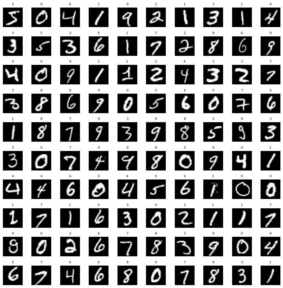
import pandas as pd

# images: [100, 1, 28, 28] from the previous snippet
flat = images.view(100, -1).numpy()  # [100, 784]

cols = [f'px_{i}' for i in range(784)]  # or [f'px_{r}_{c}' for r in range(28) for c in range(28)]
df = pd.DataFrame(flat, columns=cols)
df.insert(0, 'label', labels.numpy())

df.head()| label | px_0 | px_1 | px_2 | px_3 | px_4 | px_5 | px_6 | px_7 | px_8 | ... | px_774 | px_775 | px_776 | px_777 | px_778 | px_779 | px_780 | px_781 | px_782 | px_783 | |
|---|---|---|---|---|---|---|---|---|---|---|---|---|---|---|---|---|---|---|---|---|---|
| 0 | 5 | 0.0 | 0.0 | 0.0 | 0.0 | 0.0 | 0.0 | 0.0 | 0.0 | 0.0 | ... | 0.0 | 0.0 | 0.0 | 0.0 | 0.0 | 0.0 | 0.0 | 0.0 | 0.0 | 0.0 |
| 1 | 0 | 0.0 | 0.0 | 0.0 | 0.0 | 0.0 | 0.0 | 0.0 | 0.0 | 0.0 | ... | 0.0 | 0.0 | 0.0 | 0.0 | 0.0 | 0.0 | 0.0 | 0.0 | 0.0 | 0.0 |
| 2 | 4 | 0.0 | 0.0 | 0.0 | 0.0 | 0.0 | 0.0 | 0.0 | 0.0 | 0.0 | ... | 0.0 | 0.0 | 0.0 | 0.0 | 0.0 | 0.0 | 0.0 | 0.0 | 0.0 | 0.0 |
| 3 | 1 | 0.0 | 0.0 | 0.0 | 0.0 | 0.0 | 0.0 | 0.0 | 0.0 | 0.0 | ... | 0.0 | 0.0 | 0.0 | 0.0 | 0.0 | 0.0 | 0.0 | 0.0 | 0.0 | 0.0 |
| 4 | 9 | 0.0 | 0.0 | 0.0 | 0.0 | 0.0 | 0.0 | 0.0 | 0.0 | 0.0 | ... | 0.0 | 0.0 | 0.0 | 0.0 | 0.0 | 0.0 | 0.0 | 0.0 | 0.0 | 0.0 |
5 rows × 785 columns
Take one MNIST image. Rotate it through 0°, 1°, 2°, …, 359° → 360 points in R^784. Only one factor varies. Plot PCA(2) or t-SNE(2). You should see a closed 1-D curve (a loop). This is the canonical visualization of “rotation is a 1-D manifold in pixel space.”
import torch
import torchvision.transforms.functional as TF
import matplotlib.pyplot as plt

# Start from images[0]: shape [1, 28, 28]
img = images[0]

# Rotate by 1..360 degrees, bilinear for smoother results
angles = list(range(1, 361))
rotations = torch.stack([
    TF.rotate(img, angle=a, interpolation=TF.InterpolationMode.BILINEAR)
    for a in angles
])  # shape: [360, 1, 28, 28]

# Save the whole stack
torch.save({'rotations': rotations, 'angles': angles}, 'rotations.pt')
fig, axes = plt.subplots(18, 20, figsize=(20, 18))
for i, ax in enumerate(axes.flat):
    ax.imshow(rotations[i].squeeze(), cmap='gray')
    ax.set_title(f'{angles[i]}°', fontsize=6)
    ax.axis('off')
plt.tight_layout()
plt.savefig('rotations_grid.png', dpi=100)
plt.show()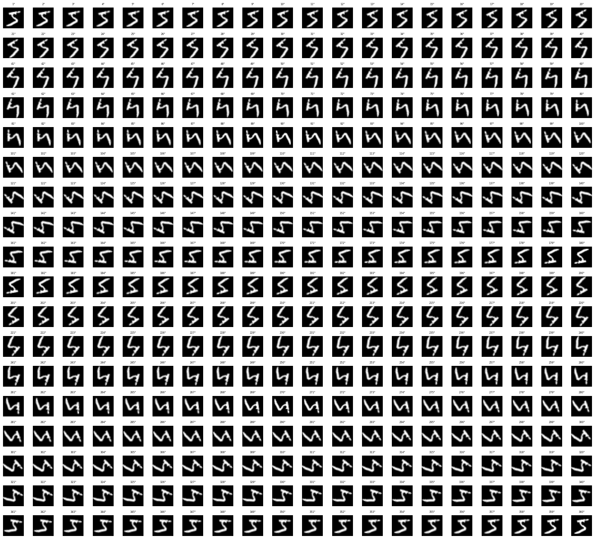
rotations.shapetorch.Size([360, 1, 28, 28])flat = rotations.view(360, -1).numpy()
cols = [f'px_{i}' for i in range(784)] # or [f'px_{r}_{c}' for r in range(28) for c in range(28)]
df = pd.DataFrame(flat, columns=cols)
df.insert(0, 'label', range(360))
df.head()| label | px_0 | px_1 | px_2 | px_3 | px_4 | px_5 | px_6 | px_7 | px_8 | ... | px_774 | px_775 | px_776 | px_777 | px_778 | px_779 | px_780 | px_781 | px_782 | px_783 | |
|---|---|---|---|---|---|---|---|---|---|---|---|---|---|---|---|---|---|---|---|---|---|
| 0 | 0 | 0.0 | 0.0 | 0.0 | 0.0 | 0.0 | 0.0 | 0.0 | 0.0 | 0.0 | ... | 0.0 | 0.0 | 0.0 | 0.0 | 0.0 | 0.0 | 0.0 | 0.0 | 0.0 | 0.0 |
| 1 | 1 | 0.0 | 0.0 | 0.0 | 0.0 | 0.0 | 0.0 | 0.0 | 0.0 | 0.0 | ... | 0.0 | 0.0 | 0.0 | 0.0 | 0.0 | 0.0 | 0.0 | 0.0 | 0.0 | 0.0 |
| 2 | 2 | 0.0 | 0.0 | 0.0 | 0.0 | 0.0 | 0.0 | 0.0 | 0.0 | 0.0 | ... | 0.0 | 0.0 | 0.0 | 0.0 | 0.0 | 0.0 | 0.0 | 0.0 | 0.0 | 0.0 |
| 3 | 3 | 0.0 | 0.0 | 0.0 | 0.0 | 0.0 | 0.0 | 0.0 | 0.0 | 0.0 | ... | 0.0 | 0.0 | 0.0 | 0.0 | 0.0 | 0.0 | 0.0 | 0.0 | 0.0 | 0.0 |
| 4 | 4 | 0.0 | 0.0 | 0.0 | 0.0 | 0.0 | 0.0 | 0.0 | 0.0 | 0.0 | ... | 0.0 | 0.0 | 0.0 | 0.0 | 0.0 | 0.0 | 0.0 | 0.0 | 0.0 | 0.0 |
5 rows × 785 columns
from sklearn.decomposition import PCA
import matplotlib.pyplot as plt
import numpy as np

# Separate features and labels
X = df.drop(columns='label').values   # (100, 784)
y = df['label'].values                # (100,)

# PCA to 2D
pca = PCA(n_components=2)
coords = pca.fit_transform(X)         # (100, 2)

print(f'Explained variance: {pca.explained_variance_ratio_}')
print(f'Total: {pca.explained_variance_ratio_.sum():.1%}')
print(f'First 10 (pairs of pairs): {pca.explained_variance_ratio_[:10]}')

# Plot, colored by digit
fig, ax = plt.subplots(figsize=(8, 6))
scatter = ax.scatter(coords[:, 0], coords[:, 1], c=y, cmap='hsv', s=40, alpha=0.8)
ax.set_xlabel(f'PC1 ({pca.explained_variance_ratio_[0]:.1%})')
ax.set_ylabel(f'PC2 ({pca.explained_variance_ratio_[1]:.1%})')
ax.set_title('PCA of rotated image')

# Discrete legend instead of a continuous colorbar
handles, _ = scatter.legend_elements()
ax.legend(handles, sorted(set(y)), title='angle of rotation', bbox_to_anchor=(1.02, 1), loc='upper left')
order = np.argsort(y)
ax.plot(coords[order, 0], coords[order, 1], '-', color='gray', alpha=0.3, linewidth=1)
plt.tight_layout()
plt.show()
Explained variance: [0.25879344 0.25624198]
Total: 51.5%
First 10 (pairs of pairs): [0.25879344 0.25624198]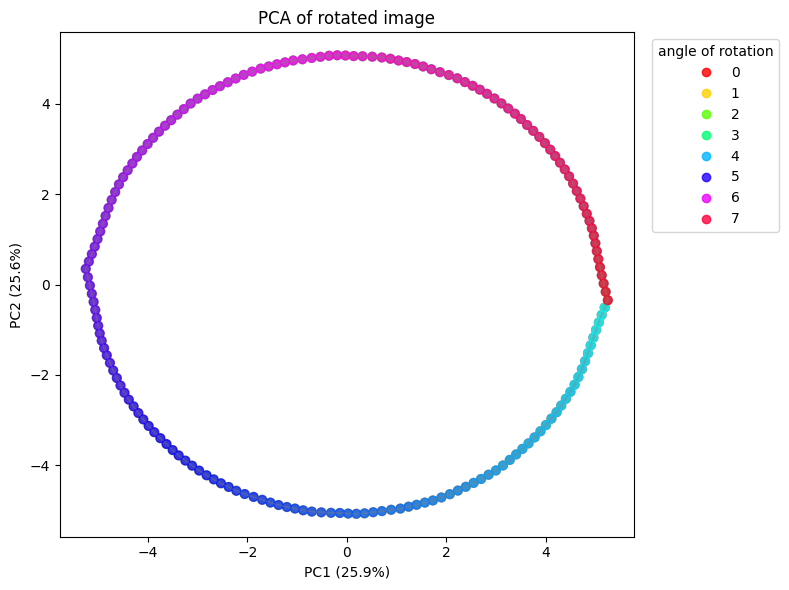
Takeaways
- total explained variance ~51.5%.
- Circular geometry is very clear.
import torch
import torch.nn as nn
from torchvision import models, transforms

# Load pretrained ResNet18, strip the classifier head
resnet = models.resnet18(weights=models.ResNet18_Weights.DEFAULT)
resnet.fc = nn.Identity()   # now returns 512-d avgpool features
resnet.eval()

# MNIST -> ResNet-ready: 1ch -> 3ch, 28x28 -> 224x224, ImageNet norm
preprocess = transforms.Compose([
    transforms.Resize(224, antialias=True),
    transforms.Normalize(mean=[0.485, 0.456, 0.406], std=[0.229, 0.224, 0.225]),
])

# rotations: [360, 1, 28, 28] in [0, 1]
x = rotations.repeat(1, 3, 1, 1)       # [360, 3, 28, 28]
x = preprocess(x)                       # [360, 3, 224, 224]

with torch.no_grad():
    embeddings = resnet(x)              # [360, 512]

print(embeddings.shape)
Downloading: "https://download.pytorch.org/models/resnet18-f37072fd.pth" to /Users/jpoberhauser/.cache/torch/hub/checkpoints/resnet18-f37072fd.pth100%|██████████| 44.7M/44.7M [00:00<00:00, 73.7MB/s]torch.Size([360, 512])
from sklearn.decomposition import PCA
import matplotlib.pyplot as plt

pca = PCA(n_components=2)
coords = pca.fit_transform(embeddings.numpy())

print(f'Explained variance: {pca.explained_variance_ratio_}')
print(f'Total: {pca.explained_variance_ratio_.sum():.1%}')

plt.figure(figsize=(7, 6))
sc = plt.scatter(coords[:, 0], coords[:, 1], c=angles, cmap='hsv', s=20)
plt.colorbar(sc, label='rotation angle (°)')
plt.xlabel(f'PC1 ({pca.explained_variance_ratio_[0]:.1%})')
plt.ylabel(f'PC2 ({pca.explained_variance_ratio_[1]:.1%})')
plt.title('PCA of ResNet18 embeddings across rotations')
plt.show()
Explained variance: [0.21693338 0.13548191]
Total: 35.2%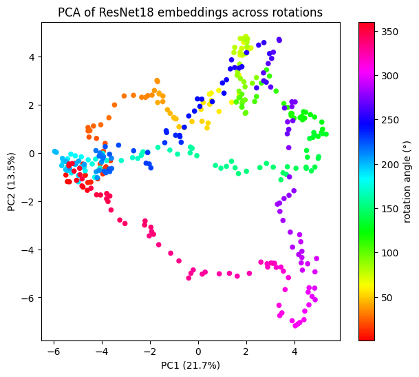
So explained vairnance went from 51 to 35%. * Top-2 PCs no longer equal → circular symmetry broke. The encoder doesn’t see rotation as an isotropic loop anymore. * The rotatoin manifold is now spread across more feature dimensions. * Resnet18 redistributed the manifold across the 512D feature space. Each feature dimension captures a different aspect of “what does the digit look like at this angle”
import torch
from torchvision import transforms

# ViT-S (22M params, 384-d output) — good default for quick experiments.
# Swap 's14' -> 'b14' (768-d), 'l14' (1024-d), or 'g14' (1536-d) for bigger models.
dinov2 = torch.hub.load('facebookresearch/dinov2', 'dinov2_vits14')
dinov2.eval()

# DINOv2 uses patch_size=14, so input H,W must be multiples of 14.
# 224 = 16*14 is the standard pretraining resolution.
preprocess = transforms.Compose([
    transforms.Resize(224, antialias=True),
    transforms.Normalize(mean=[0.485, 0.456, 0.406], std=[0.229, 0.224, 0.225]),
])

# rotations: [360, 1, 28, 28]
x = rotations.repeat(1, 3, 1, 1)   # [360, 3, 28, 28]
x = preprocess(x)                   # [360, 3, 224, 224]

with torch.no_grad():
    embeddings = dinov2(x)          # [360, 384] — CLS token

print(embeddings.shape)
Using cache found in /Users/jpoberhauser/.cache/torch/hub/facebookresearch_dinov2_main
/Users/jpoberhauser/.cache/torch/hub/facebookresearch_dinov2_main/dinov2/layers/swiglu_ffn.py:51: UserWarning: xFormers is not available (SwiGLU)
warnings.warn("xFormers is not available (SwiGLU)")
/Users/jpoberhauser/.cache/torch/hub/facebookresearch_dinov2_main/dinov2/layers/attention.py:33: UserWarning: xFormers is not available (Attention)
warnings.warn("xFormers is not available (Attention)")
/Users/jpoberhauser/.cache/torch/hub/facebookresearch_dinov2_main/dinov2/layers/block.py:40: UserWarning: xFormers is not available (Block)
warnings.warn("xFormers is not available (Block)")torch.Size([360, 384])from sklearn.decomposition import PCA
import matplotlib.pyplot as plt
coords = PCA(n_components=2).fit_transform(embeddings.numpy())
pca = PCA(n_components=2)
coords = pca.fit_transform(embeddings.numpy())
print(f'Explained variance: {pca.explained_variance_ratio_}')
print(f'Total: {pca.explained_variance_ratio_.sum():.1%}')
plt.figure(figsize=(7, 6))
sc = plt.scatter(coords[:, 0], coords[:, 1], c=angles, cmap='hsv', s=20)
plt.colorbar(sc, label='rotation angle (°)')
plt.title('PCA of DINOv2 embeddings across rotations')
plt.show()Explained variance: [0.33095375 0.16032468]
Total: 49.1%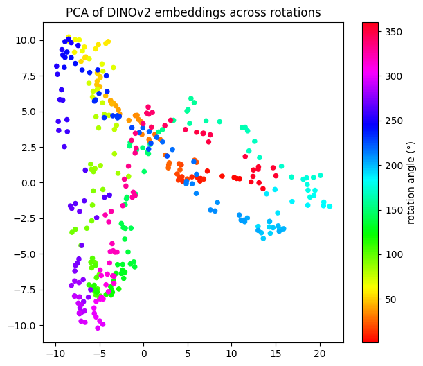
Wrapping up all three results:
  ┌───────────────────────┬───────┬───────┬───────┬───────────────┬────────────────────────────────┐
  │         Space         │  PC1  │  PC2  │ Total │ PC1/PC2 ratio │            Geometry            │
  ├───────────────────────┼───────┼───────┼───────┼───────────────┼────────────────────────────────┤
  │ Pixel                 │ 25.9% │ 25.6% │ 51.5% │ 1.01          │ Curved + circular              │
  ├───────────────────────┼───────┼───────┼───────┼───────────────┼────────────────────────────────┤
  │ ResNet18 (supervised) │ 21.7% │ 13.5% │ 35.2% │ 1.61          │ Spread thin, mildly elliptical │
  ├───────────────────────┼───────┼───────┼───────┼───────────────┼────────────────────────────────┤
  │ DINOv2 (SSL)          │ 33.1% │ 16.0% │ 49.1% │ 2.07          │ Stretched, dominant axis       │
  └───────────────────────┴───────┴───────┴───────┴───────────────┴────────────────────────────────┘
Takeaways
- The manifold hypothesis on prior 6 is empircaly real and shown in the eexercies above.
- Recall: prior 6 –> 6. manifold hypothesis: data concentrated in a low-dimensional manifold in high-dimension input ambient space. The intrinsic dimension of the manifold is the number of underlying factors. This is why KNN works on SSL features but not on raw pixels. So if we have one factor of variatoin (angle), then there is one intrinsic dimension of the structure of the data, regardless of the 784 input space.
- Off the shelf supervised encoder like resnet18 reshapes that manifold.
Exercise 2 — Invariance vs equivariance, empirically
Take the same pretrained ResNet18. For a single image, compute: - g(x) — features of the original image, - g(T x) — features of a translated copy (shift by 16 pixels), - g(R x) — features of a rotated copy (90°).
Compute cosine similarity for each pair. Is the network more invariant to translation or rotation? Why? (Hint: think about the training data and the architecture.)
# TODO
# 1. one image (any image, even a single PIL load)
# 2. compute features for x, shift(x, 16), rotate(x, 90)
# 3. cosine sims
# 4. one-sentence observation below
Exercise 3 — The collapse problem, by hand
No training. Just construct two encoders g_A and g_B mapping R^d -> R^k:
g_A(x) = 0for allx(the trivial collapsed solution).g_B(x) = W xwithWa random projection.
Both are perfectly smooth. Both are perfectly invariant to noise. Yet only one is useful.
Write 2–3 sentences: which of Bengio’s priors does g_A violate? Which of LeCun’s EBM constraints rules it out?
Your answer:
…
End-of-week recap
Write a ≤200-word summary you could send to a colleague who hasn’t read either paper. Cover: 1. What a representation is and why we want one separate from the predictor. 2. Bengio’s priors — pick the 3 you think matter most for image SSL. 3. LeCun’s argument for SSL over supervised. 4. The one open question you most want to follow up on.
…
Next week (Phase 1 / Week 2): information-theoretic view — mutual information, InfoNCE bound, why MI bounds are loose in practice. Tschannen et al., Oord et al., Poole et al.